Distributed Cox Regression
Introduction
It is only a short way from the toy MLE example to a more useful example using Cox regression.
But first, we need the survival package.
if (!require("survival")) {
    stop("this vignette requires the survival package")
}
We generate some simulated data for the purpose of this example. We will have three sites each with patient data (sizes 1000, 500 and 1500) respectively, containing
sex(0, 1) for male/femaleagebetween 40 and 70- a biomarker
bm - a
timeto some event of interest - an indicator
eventwhich is 1 if an event was observed and 0 otherwise.
It is common to fit stratified models using sites as strata since the patient characteristics usually differ from site to site. So the baseline hazards (lambdaT) are different for each site but they share common coefficients (beta.1, beta.2 and beta.3 for age, sex and bm respy.) for the model. See (Terry M. Therneau and Patricia M. Grambsch 2000) by Therneau and Grambsch for details. So our model for each site \(i\) is
\[ S(t, age, sex, bm) = [S_0^i(t)]^{\exp(\beta_1 age + \beta_2 sex + \beta_3 bm)} \]
sampleSize <- c(n1 = 1000, n2 = 500, n3 = 1500)

set.seed(12345)

beta.1 <- -.015; beta.2 <- .2; beta.3 <- .001;

lambdaT <- c(5, 4, 3)
lambdaC <- 2

coxData <- lapply(seq_along(sampleSize),
                  function(i) {
                      sex <- sample(c(0, 1), size = sampleSize[i], replace = TRUE)
                      age <- sample(40:70, size = sampleSize[i], replace = TRUE)
                      bm <- rnorm(sampleSize[i])
                      trueTime <- rweibull(sampleSize[i],
                                           shape = 1,
                                           scale = lambdaT[i] * exp(beta.1 * age + beta.2 * sex + beta.3 * bm ))
                      censoringTime <- rweibull(sampleSize[i],
                                                shape = 1,
                                                scale = lambdaC)
                      time <- pmin(trueTime, censoringTime)
                      event <- (time == trueTime)
                      data.frame(stratum = i,
                                 sex = sex,
                                 age = age,
                                 bm = bm,
                                 time = time,
                                 event = event)
                  })
So here is a summary of the data for the three sites.
Site 1
str(coxData[[1]])## 'data.frame': 1000 obs. of 6 variables:
## $ stratum: int 1 1 1 1 1 1 1 1 1 1 ...
## $ sex : num 1 1 1 1 0 0 0 1 1 1 ...
## $ age : int 42 66 40 50 61 47 45 61 70 69 ...
## $ bm : num 1.6775 0.0795 -0.8564 -0.7788 -0.3809 ...
## $ time : num 3.42 1.051 0.509 2.868 1.073 ...
## $ event : logi FALSE TRUE TRUE TRUE FALSE TRUE ...Site 2
str(coxData[[2]])## 'data.frame': 500 obs. of 6 variables:
## $ stratum: int 2 2 2 2 2 2 2 2 2 2 ...
## $ sex : num 1 0 0 0 0 1 0 1 1 0 ...
## $ age : int 67 43 48 47 45 55 52 57 54 69 ...
## $ bm : num -0.225 -0.527 -0.642 1.717 1.323 ...
## $ time : num 3.409 0.766 0.075 1.637 0.471 ...
## $ event : logi TRUE TRUE FALSE TRUE FALSE FALSE ...Site 3
str(coxData[[3]])## 'data.frame': 1500 obs. of 6 variables:
## $ stratum: int 3 3 3 3 3 3 3 3 3 3 ...
## $ sex : num 1 1 0 0 1 0 0 1 1 0 ...
## $ age : int 42 64 42 47 48 43 54 59 52 63 ...
## $ bm : num -0.349 -1.026 -0.907 0.775 -0.95 ...
## $ time : num 4.893 1.076 0.37 3.192 0.144 ...
## $ event : logi FALSE TRUE TRUE TRUE FALSE FALSE ...Aggregated fit
If the data were all aggregated in one place, it would very simple to fit the model. Below, we row-bind the data from the three sites.
aggModel <- coxph(formula = Surv(time, event) ~ sex +
                                age + bm + strata(stratum),
                            data = do.call(rbind, coxData))
aggModel
## Call:
## coxph(formula = Surv(time, event) ~ sex + age + bm + strata(stratum),
## data = do.call(rbind, coxData))
##
## coef exp(coef) se(coef) z p
## sex -0.17959 0.83562 0.05069 -3.54 0.0004
## age 0.02009 1.02029 0.00286 7.02 2.1e-12
## bm 0.00682 1.00684 0.02501 0.27 0.7852
##
## Likelihood ratio test=61.9 on 3 df, p=2.32e-13
## n= 3000, number of events= 1588Here age and sex are significant, but bm is not. The estimates \(\hat{\beta}\) are (-0.180, .020, .007).
We can also print out the value of the (partial) log-likelihood at the MLE.
aggModel$loglik## [1] -9594.620 -9563.676The first is the value at the parameter value (0, 0, 0) and the last is the value at the MLE.
Distributed Computation
Assume now that the data coxData is distributed between three sites none of whom want to share actual data among each other or even with a master computation process. They wish to keep their data secret but are willing, together, to provide the sum of their local negative log-likelihoods. They need to do this in a way so that the master process will not be able to associate the contribution to the likelihood from each site.
The overall likelihood function \(l(\lambda)\) for the entire data is therefore the sum of the likelihoods at each site: \(l(\lambda) = l_1(\lambda)+l_2(\lambda)+l_3(\lambda).\) How can this likelihood be computed while maintaining privacy?
Assuming that every site including the master has access to a homomorphic computation library such as homomorpheR, the likelihood can be computed in a privacy-preserving manner using the following scheme. We use \(E(x)\) and \(D(x)\) to denote the encrypted and decrypted values of \(x\) respectively.
- Master generates a public/private key pair. Master distributes the public key to all sites. (The private key is not distributed and kept only by the master.)
- Master generates a random offset \(r\) to obfuscate the intial likelihood.
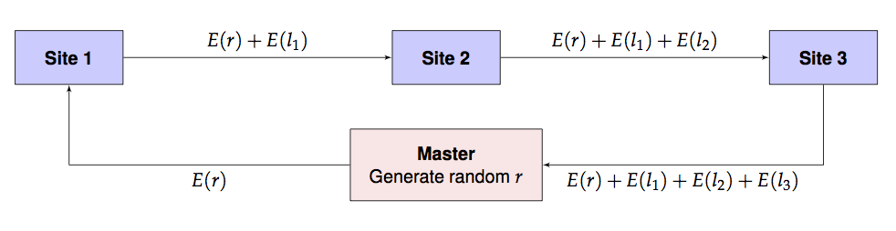
- Master sends \(E(r)\) and a guess \(\lambda_0\) to site 1. Note that \(\lambda\) is not encrypted.
- Site 1 computes \(l_1 = l(\lambda_0, y_1)\), the local likelihood for local data \(y_1\) using parameter \(\lambda_0\). It then sends on \(\lambda_0\) and \(E(r) + E(l_1)\) to site 2.
- Site 2 computes \(l_2 = l(\lambda_0, y_2)\), the local likelihood for local data \(y_2\) using parameter \(\lambda_0\). It then sends on \(\lambda_0\) and \(E(r) + E(l_1) + E(l_2)\) to site 3.
- Site 3 computes \(l_3 = l(\lambda_0, y_3)\), the local likelihood for local data \(y_3\) using parameter \(\lambda_0\). It then sends on \(E(r) + E(l_1) + E(l_2) + E(l_3)\) back to master.
- Master retrieves \(E(r) + E(l_1) + E(l_2) + E(l_3)\) which, due to the homomorphism, is exactly \(E(r+l_1+l_2+l_3) = E(r+l).\) So the master computes \(D(E(r+l)) - r\) to obtain the value of the overall likelihood at \(\lambda_0\).
- Master updates \(\lambda_0\) with a new guess \(\lambda_1\) and repeats steps 1-5. This process is iterated to convergence. For added security, even steps 0-5 can be repeated, at additional computational cost.
This is pictorially shown below.
Implementation
The above implementation assumes that the encryption and decryption can happen with real numbers which is not the actual situation. Instead, we use rational approximations using a large denominator, \(2^{256}\), say. In the future, of course, we need to build an actual library is built with rigorous algorithms guaranteeing precision and overflow/undeflow detection. For now, this is just an ad hoc implementation.
Also, since we are only using homomorphic additive properties, a partial homomorphic scheme such as the Paillier Encryption system will be sufficient for our computations.
We define a class to encapsulate our sites that will compute the Poisson likelihood on site data given a parameter \(\lambda\). Note how the addNLLAndForward method takes care to split the result into an integer and fractional part while performing the arithmetic operations. (The latter is approximated by a rational number.)
We define a class to encapsulate our sites that will compute the partial log likelihood on site data given a parameter \(\beta\).
In the code below, we exploit, for expository purposes, a feature of coxph: a control parameter can be passed to evaluate the partial likelihood at a given \(\beta\) value.
library(gmp)
library(homomorpheR)
Site <- R6::R6Class("Site",
                    private = list(
                        ## name of the site
                        name = NA,
                        ## only master has this, NA for workers
                        privkey = NA,
                        ## local data
                        data = NA,
                        ## The next site in the communication: NA for master
                        nextSite = NA,
                        ## is this the master site?
                        iAmMaster = FALSE,
                        ## intermediate result variable
                        intermediateResult = NA,
                        ## Control variable for cox regression
                        cph.control = NA
                    ),
                    public = list(
                        count = NA,
                        ## Common denominator for approximate real arithmetic
                        den = NA,
                        ## The public key; everyone has this
                        pubkey = NA,
                        initialize = function(name, data, den) {
                            private$name <- name
                            private$data <- data
                            self$den <- den
                            private$cph.control <- replace(coxph.control(), "iter.max", 0)
                        },
                        setPublicKey = function(pubkey) {
                            self$pubkey <- pubkey
                        },
                        setPrivateKey = function(privkey) {
                            private$privkey <- privkey
                        },
                        ## Make me master
                        makeMeMaster = function() {
                            private$iAmMaster <- TRUE
                        },
                        ## add neg log lik and forward to next site
                        addNLLAndForward = function(beta, enc.offset) {
                            if (private$iAmMaster) {
                                ## We are master, so don't forward
                                ## Just store intermediate result and return
                                private$intermediateResult <- enc.offset
                            } else {
                                ## We are workers, so add and forward
                                ## add negative log likelihood and forward result to next site
                                ## Note that offset is encrypted
                                nllValue <- self$nLL(beta)
                                result.int <- floor(nllValue)
                                result.frac <- nllValue - result.int
                                result.fracnum <- as.bigq(numerator(as.bigq(result.frac) * self$den))
                                pubkey <- self$pubkey
                                enc.result.int <- pubkey$encrypt(result.int)
                                enc.result.fracnum <- pubkey$encrypt(result.fracnum)
                                result <- list(int = pubkey$add(enc.result.int, enc.offset$int),
                                               frac = pubkey$add(enc.result.fracnum, enc.offset$frac))
                                private$nextSite$addNLLAndForward(beta, enc.offset = result)
                            }
                            ## Return a TRUE result for now.
                            TRUE
                        },
                        ## Set the next site in the communication graph
                        setNextSite = function(nextSite) {
                            private$nextSite <- nextSite
                        },
                        ## The negative log likelihood
                            nLL = function(beta) {
                            if (private$iAmMaster) {
                                ## We're master, so need to get result from sites
                                ## 1. Generate a random offset and encrypt it
                                pubkey <- self$pubkey
                                offset <- list(int = random.bigz(nBits = 256),
                                               frac = random.bigz(nBits = 256))
                                enc.offset <- list(int = pubkey$encrypt(offset$int),
                                                   frac = pubkey$encrypt(offset$frac))
                                ## 2. Send off to next site
                                throwaway <- private$nextSite$addNLLAndForward(beta, enc.offset)
                                ## 3. When the call returns, the result will be in
                                ##    the field intermediateResult, so decrypt that.
                                sum <- private$intermediateResult
                                privkey <- private$privkey
                                intResult <- as.double(privkey$decrypt(sum$int) - offset$int)
                                fracResult <- as.double(as.bigq(privkey$decrypt(sum$frac) - offset$frac) / den)
                                intResult + fracResult
                            } else {
                                ## We're worker, so compute local negative log likelihood
                                tryCatch({
                                    m <- coxph(formula = Surv(time, event) ~ sex + age + bm,
                                                         data = private$data,
                                                         init = beta,
                                                         control = private$cph.control)
                                    -(m$loglik[1])
                                },
                                error = function(e) NA)
                            }
                        })
                    )
We are now ready to use our sites in the computation.
1. Generate public and private key pair
We also choose a denominator for all our rational approximations.
keys <- PaillierKeyPair$new(1024) ## Generate new public and private key.
den <- gmp::as.bigq(2)^256  #Our denominator for rational approximations
2. Create sites
site1 <- Site$new(name = "Site 1", data = coxData[[1]], den = den)
site2 <- Site$new(name = "Site 2", data = coxData[[2]], den = den)
site3 <- Site$new(name = "Site 3", data = coxData[[3]], den = den)
The master process is also a site but has no data. So has to be thus designated.
## Master has no data!
master <- Site$new(name = "Master", data = c(), den = den)
master$makeMeMaster()
2. Distribute public key to sites
site1$setPublicKey(keys$pubkey)
site2$setPublicKey(keys$pubkey)
site3$setPublicKey(keys$pubkey)
master$setPublicKey(keys$pubkey)
Only master has private key for decryption.
master$setPrivateKey(keys$getPrivateKey())3. Define the communication graph
Master will always send to the first site, and then the others have to forward results in turn with the last site returning to the master.
master$setNextSite(site1)
site1$setNextSite(site2)
site2$setNextSite(site3)
site3$setNextSite(master)
4. Perform the likelihood estimation
library(stats4)
nll <- function(age, sex, bm) master$nLL(c(age, sex, bm))
fit <- mle(nll, start = list(age = 0, sex = 0, bm = 0))
5. Compare the results
The summary will show the results, but only the coefficients and the standard errors.
summary(fit)## Maximum likelihood estimation
##
## Call:
## mle(minuslogl = nll, start = list(age = 0, sex = 0, bm = 0))
##
## Coefficients:
## Estimate Std. Error
## age -0.179585179 0.050694606
## sex 0.020087782 0.002859509
## bm 0.006815326 0.025006028
##
## -2 log L: 19127.35Let us recreate a summary table similar to what would be produced by the summary call on the aggregated model, for comparison.
ourSummary <- function(fit) {
    coefs <- coef(fit)
    se <- sqrt(diag(vcov(fit)))
    expCoef <- exp(coefs)
    zScore <- coefs / se
    pValue <- 2 * pnorm(abs(coefs / se), lower.tail = FALSE)
    result <- cbind(coefs, expCoef, se, zScore, pValue)
    colnames(result) <- c("coef", "exp(coef)", "se(coef)", "z", "Pr(>|z|)")
    result
}
print(ourSummary(fit), digits = 4)
## coef exp(coef) se(coef) z Pr(>|z|)
## age -0.179585 0.8356 0.05069 -3.5425 3.964e-04
## sex 0.020088 1.0203 0.00286 7.0249 2.142e-12
## bm 0.006815 1.0068 0.02501 0.2725 7.852e-01Note how the estimated coefficients and standard errors closely match the full model summary below.
summary(aggModel)## Call:
## coxph(formula = Surv(time, event) ~ sex + age + bm + strata(stratum),
## data = do.call(rbind, coxData))
##
## n= 3000, number of events= 1588
##
## coef exp(coef) se(coef) z Pr(>|z|)
## sex -0.179585 0.835617 0.050695 -3.542 0.000396 ***
## age 0.020088 1.020291 0.002859 7.025 2.14e-12 ***
## bm 0.006815 1.006839 0.025006 0.273 0.785204
## ---
## Signif. codes: 0 '***' 0.001 '**' 0.01 '*' 0.05 '.' 0.1 ' ' 1
##
## exp(coef) exp(-coef) lower .95 upper .95
## sex 0.8356 1.1967 0.7566 0.9229
## age 1.0203 0.9801 1.0146 1.0260
## bm 1.0068 0.9932 0.9587 1.0574
##
## Concordance= 0.563 (se = 0.013 )
## Rsquare= 0.02 (max possible= 0.998 )
## Likelihood ratio test= 61.89 on 3 df, p=2.323e-13
## Wald test = 61.71 on 3 df, p=2.528e-13
## Score (logrank) test = 62.04 on 3 df, p=2.156e-13And the log likelihood of the distributed homomorphic fit also matches as the following computation shows.
## -2 Log L
-2 * logLik(fit)
## 'log Lik.' 19127.35 (df=3)Other Topologies
Another communication strategy is to pair each worker with a neighbor.
- Each site \(i\) sends \(E(l_i + r_i)\) and \(E(l_i - r_i)\) to its neighbor workers.
- In a synchronization step, all workers sum up what they got from their neighbors.
- Master then queries each worker which responds the sum.
- Master sums all of these together.
References
Terry M. Therneau, and Patricia M. Grambsch. 2000. Modeling Survival Data: Extending the Cox Model. New York: Springer-Verlag.